SymPy Demo 4: The Eigenvalue Problem

SymPy Demo 4: The Eigenvalue Problem#

Demo by Christian Mikkelstrup og Hans Henrik Hermansen, Karl Johan Måstrup Kristiansen, and Magnus Troen. Revised 11-11-24 by shsp.

from sympy import *
init_printing()

In this demo we wish to show how to manipulate a matrix for the purpose of solving the eigenvalue problem (finding eigenvectors and eigenvalues as well as other associated properties).

We will be working on the mapping matrix

\[\begin{split} _e[\boldsymbol f]_e = \begin{bmatrix}6&3&12\\4&-5&4\\-4&-1&-10\end{bmatrix}, \end{split}\]

which represents the linear map \(\boldsymbol f:\mathbb{R}^3\to \mathbb{R}^3\) with respect to the standard basis. See the course textbook for all the details about definitions, notation, terminology, and theorems, whcih we will be using freely in the following.

eFe = Matrix([[6,3,12],[4,-5,4],[-4,-1,-10]])

Eigenvalues#

The characteristic matrix \(\mathbf K(\lambda)= ~_e[\boldsymbol f]_e-\lambda\cdot \mathbf I_3\) is constructed as follows:

lamb = symbols('\lambda')
K = eFe - lamb * eye(3)
K

\[\begin{split}\displaystyle \left[\begin{matrix}6 - \lambda & 3 & 12\\4 & - \lambda - 5 & 4\\-4 & -1 & - \lambda - 10\end{matrix}\right]\end{split}\]

The characteristic polynomial is its determinant, \(p(\lambda)=\mathrm{det}(\mathbf K(\lambda))\):

charpoly = K.det()
charpoly

../_images/ac6f41a25167cd6e7ef8af1f54a3a09341406c7225b2ff345d3ba4023c5aebb6.png

A SymPy command can do this in one step, but note that the sign here is different. This is not a problem, though, since we are interested in the roots of this polynomial.

eFe.charpoly()

../_images/4a52691766f1fde3c1993635cd238a68a598b005db2da0777d34f359ceca3bcb.png

The characteristic equation is the characteristic polynomial set equal to zero, \(\mathrm{det}(\mathbf K(\lambda))=0\):

chareq = Eq(charpoly, 0)
chareq

../_images/6212ea07929209027448cc519960bdea450d875f68848f17d18b1ed7a5e1a876.png

The eigenvalues of the original mapping matrix can now be found either by solving the characteristic equation or by using SymPy’s command .roots() to find the roots in the characteristic polynomial:

roots(charpoly)

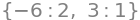
../_images/766c12294a627cfbdec29ce99436aa90b7215510c7fa6dd21a3ea67d317e1e70.png

solveset(chareq, lamb)

../_images/2860f9375580a04c0b916e23ae1f722cb698f9ce42147d6388dcdf6c2ff18705.png

Note that solveset() does not catch the fact that \(-6\) has an algebraic multiplicity of \(2\)! If we do not want to miss the multiplicity, then we can ask SymPy for the factorisation as shown below, but often roots() is more convenient in such cases.

factor(charpoly)

../_images/4c335e81d49f9c94f6f65e9f0c9f3937b59bf1dd10602cba473719bcbf66f722.png

Eigenvectors#

Finding the eigenvectors belonging to the eigenvalue \(-6\) means solving the equation \(\mathbf K(-6)\,\mathbf x=\mathbf{0}\). We find \(\mathbf K(-6)\) as follows:

K.subs(lamb, -6)

\[\begin{split}\displaystyle \left[\begin{matrix}12 & 3 & 12\\4 & 1 & 4\\-4 & -1 & -4\end{matrix}\right]\end{split}\]

We solve using the above coefficient matrix with a right-hand side of zeros:

K.subs(lamb, -6).gauss_jordan_solve(zeros(3,1))

\[\begin{split}\displaystyle \left( \left[\begin{matrix}- \frac{\tau_{0}}{4} - \tau_{1}\\\tau_{0}\\\tau_{1}\end{matrix}\right], \ \left[\begin{matrix}\tau_{0}\\\tau_{1}\end{matrix}\right]\right)\end{split}\]

We see from the output two linearly independent eigenvectors of our map. They span the eigenspace for the eigenvalue \(-6\). This eigenspace can hence be written as:

\[\begin{split} E_{-6}=\text{span}\left(\begin{bmatrix}-\frac{1}{4} \\ 1\\ 0 \end{bmatrix}, \begin{bmatrix} -1\\ 0\\ 1\end{bmatrix}\right). \end{split}\]

We count the geometric multiplicity to be \(2\) (the dimension of the eigenspace) for this eigenvalue of \(-6\).

Eigenvectors associated with the eigenvalue of \(3\) are likewise found by solving \(\mathbf K(3)\,x=\mathbf{0}\), which the readers might notice is the same is finding the kernel, \(\ker \mathbf K(3).\)

K.subs(lamb, 3).nullspace()

\[\begin{split}\displaystyle \left[ \left[\begin{matrix}-3\\-1\\1\end{matrix}\right]\right]\end{split}\]

From this we see that \(E_3=\text{span}((-3,-1,1))\) and that the geometric multiplicity is equal to the algebraic multiplicity, namely \(1\).

Built-in Commands for finding Eigenvalues and -Vectors#

There actually is no need for dealing with characteristic matrices, characteristic polynomials, and characteristic equations etc. in a manual manner as we did above, because SymPy comes with built-in commands that you can apply directly on the mapping matrix. Typically, the only reason for the above would be if you need to meticulously look through the steps, or if you need an intermediate output. If that’s not relevant, then you can very quickly solve the eigenproblem with the following:

eFe.eigenvals()

eFe.eigenvects()

\[\begin{split}\displaystyle \left[ \left( -6, \ 2, \ \left[ \left[\begin{matrix}- \frac{1}{4}\\1\\0\end{matrix}\right], \ \left[\begin{matrix}-1\\0\\1\end{matrix}\right]\right]\right), \ \left( 3, \ 1, \ \left[ \left[\begin{matrix}-3\\-1\\1\end{matrix}\right]\right]\right)\right]\end{split}\]

In fact, .eigenvects() provides you with all data in one go - both the eigenvalues, their algebraic multiplicities, and associated (linearly independent) eigenvectors! The output format that you see above is the following:

\[\left[\Bigl(\lambda_1, \quad \operatorname {am}(\lambda_1),\quad \verb|eigenvectors for |\lambda_1\Bigr), \Bigl(\lambda_2, \quad \operatorname {am}(\lambda_2),\quad \verb|eigenvectors for |\lambda_2\Bigr),\ \ldots\right].\]

Each bracket in the output displays info related to each unique eigenvalue.

You might infer that you still are missing one piece of info: what about the geometric multiplicity for each eigenvalue? But in fact that is also clear from the output, since that is just the number of (linearly independent) eigenvectors associated with an eigenvalue, which is easy to count from the output. And the eigenspaces can be written as the span of the shown eigenvectors for each eigenvalue.

You can automate the process of extracting this data from the output as follows:

eigen_info = eFe.eigenvects()

for lmb, am_lmb, list_of_v in eigen_info:
    print(f'For the eigenvalue {lmb} with algebraic multiplicity {am_lmb}, the eigenspace is spanned by the eigenvectors')
    display(list_of_v)
    print(f'and the geometric multiplicity is {len(list_of_v)}' + '\n\n')

For the eigenvalue -6 with algebraic multiplicity 2, the eigenspace is spanned by the eigenvectors

\[\begin{split}\displaystyle \left[ \left[\begin{matrix}- \frac{1}{4}\\1\\0\end{matrix}\right], \ \left[\begin{matrix}-1\\0\\1\end{matrix}\right]\right]\end{split}\]

and the geometric multiplicity is 2

For the eigenvalue 3 with algebraic multiplicity 1, the eigenspace is spanned by the eigenvectors